Let's Talk About DBSCAN and OPTICS Clustering Algorithms
section-content
section-content
Let's Talk About DBSCAN and OPTICS Clustering Algorithms
Today, we'll discuss two popular clustering algorithms: DBSCAN and OPTICS. We'll look at their features and compare them.
TL;DR
For the impatient:
-
[Worst-case runtime: O(n2)O(n²)O(n2), but can improve to O(nlogn)O(n \log n)O(nlogn) with spatial indexing (e.g., KD-trees or R-trees).]
-
[Requires two parameters: ε\varepsilonε (neighborhood radius) and minPts (minimum points to form a cluster).]
-
[Good for datasets with well-defined dense regions and noise.]
-
[Struggles with clusters of varying density due to fixed ε\varepsilonε.]
-
[Optimized version has a runtime of O(nlogn)O(n \log n)O(nlogn) with spatial indexing but can be slower due to reachability plot construction.]
-
[More complex to implement, includes an additional step of ordering points by reachability.]
-
[Suitable for datasets with clusters of varying densities.]
-
[Uses the same parameters (ε\varepsilonε and minPts) but is less sensitive to ε\varepsilonε.]
-
[More flexible with varying density clusters.]
Detailed Explanation of DBSCAN
DBSCAN (Density-based spatial clustering of applications with noise) works by grouping points that are closely packed together and marking points in low-density regions as noise. It requires a proximity matrix and two parameters: the radius ε and the minimum number of neighbors minPts.
Here's an example implementation using Python and Sci-Kit Learn:
import pandas as pd
import matplotlib.pyplot as plt
from sklearn.cluster import DBSCAN
from sklearn.preprocessing import StandardScaler
from ipywidgets import interact
data = pd.read_csv('distribution-2.csv', header=None)
## Normalize data
scaler = StandardScaler()
scaled_data = scaler.fit_transform(data)
@interact(epsilon=(0, 1.0, 0.05), min_samples=(5, 10, 1))
def plot_dbscan(epsilon, min_samples):
dbscan = DBSCAN(eps=epsilon, min_samples=min_samples)
clusters = dbscan.fit_predict(scaled_data)
plt.figure(figsize=(6, 4), dpi=150)
plt.scatter(data[0], data[1], c=clusters, cmap='viridis', s=40, alpha=1, edgecolors='k')
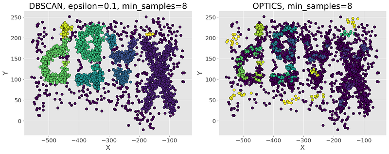
plt.title('DBSCAN')
plt.xlabel('X')
plt.ylabel('Y')
plt.show()
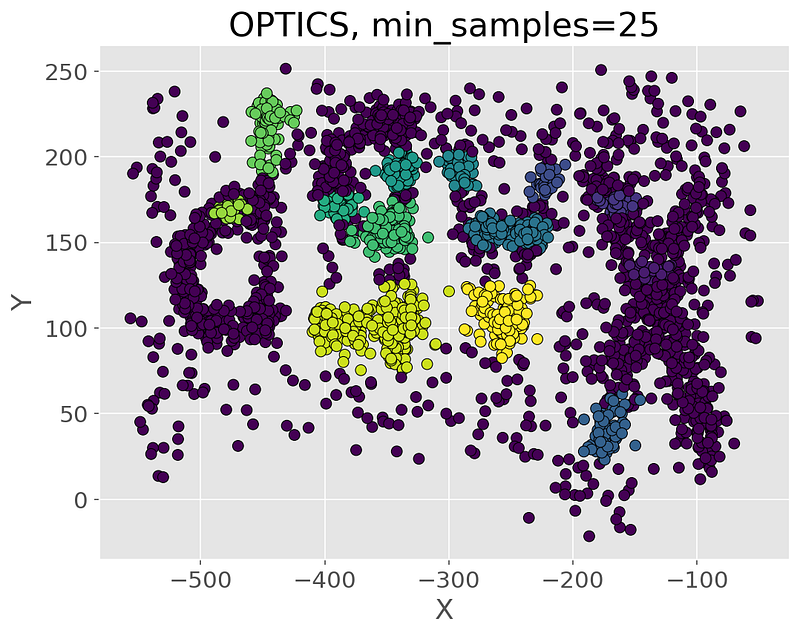
Detailed Explanation of OPTICS

OPTICS (Ordering Points To Identify the Clustering Structure) is similar to DBSCAN but better suited for datasets with varying densities. It uses a reachability plot to order points and determine the reachability distance for clustering.
Example implementation in Python:
import pandas as pd
import matplotlib.pyplot as plt
from sklearn.cluster import OPTICS
from sklearn.preprocessing import StandardScaler

data = pd.read_csv('distribution.csv', header=None)

## Normalize data
scaler = StandardScaler()
scaled_data = scaler.fit_transform(data)

min_samples = 25
optics = OPTICS(min_samples=min_samples)
clusters = optics.fit_predict(scaled_data)

plt.figure(figsize=(8, 6))
plt.scatter(data[0], data[1], c=clusters, cmap='viridis', s=50, alpha=1, edgecolors='k')
plt.title(f'OPTICS, ')
plt.xlabel('X')
plt.ylabel('Y')
plt.show()
Comparison of DBSCAN and OPTICS
- [Pros:]
- [Does not require specifying the number of clusters.]
- [Finds clusters of arbitrary shape.]
- [Resistant to noise and outliers.]
- [Cons:]
- [Sensitive to the choice of ε\varepsilonε.]
- [Struggles with varying density clusters.]
Pros:
Identifies clusters with varying densities.
Does not require specifying the number of clusters.
Resistant to noise.
Cons:
More complex to implement.
Can be slower due to the reachability plot construction.


I hope this overview has been helpful!
Written by
Anton Vice