How to Train a KAN Model on the Titanic Dataset for Kaggle
How to Train a KAN Model on the Titanic Dataset for Kaggle
CHECKOUT LIKE AND SUBSCRIBE TO MY FINAL SUBMISSION WITH [Score: 0.77751] here https://www.kaggle.com/code/dzehtsiarou/better-kan-titenic
YES WE KAN!
Introduction
Training machine learning models on real-world datasets is an exciting yet challenging task. The Titanic dataset on Kaggle is a great starting point for beginners to explore and practice predictive modeling. In this blog post, I will guide you through the steps to train a Knowledge Augmented Network (KAN) model on the Titanic dataset. This tutorial will cover data preprocessing, model training, and making predictions for Kaggle submission.
Step-by-Step Guide
Step 1: Import Necessary Libraries
First, we need to import essential libraries for data manipulation, model training, and preprocessing.
import pandas as pd
import torch
import numpy as np
from sklearn.preprocessing import LabelEncoder, StandardScaler
from sklearn.model_selection import train_test_split
Step 2: Load the Data
We load the training and test datasets from CSV files provided by Kaggle.
train_data = pd.read_csv('/kaggle/input/titanic/train.csv')
test_data = pd.read_csv('/kaggle/input/titanic/test.csv')
Step 3: Encode Categorical Variables
Next, we convert categorical columns to numerical format using
LabelEncoder.
label_encoder = LabelEncoder()
for col in ['Name', 'Sex', 'Ticket']:
    train_data[col] = label_encoder.fit_transform(train_data[col])
    test_data[col] = label_encoder.fit_transform(test_data[col])
Step 4: Fill Missing Values
To handle missing data, we replace missing values in numeric columns with the column mean.
train_data.fillna(train_data.select_dtypes(include=[np.number]).mean(), inplace=True)
test_data.fillna(test_data.select_dtypes(include=[np.number]).mean(), inplace=True)
Step 5: Prepare Features and Target Variables
We prepare the features and target variables by dropping unnecessary columns and separating features from the target variable.
train_df = train_data.drop(['PassengerId', 'Survived', 'Age', 'Cabin', 'Embarked'], axis=1)
target_df = train_data['Survived']
Step 6: Split the Data
We split the data into training and test sets using
train_test_split.
X_train, X_test, y_train, y_test = train_test_split(train_df, target_df, test_size=0.2, random_state=42)
Step 7: Normalize the Data
Standardizing the feature data helps in stabilizing and speeding up the training process.
scaler = StandardScaler()
X_train_scaled = scaler.fit_transform(X_train)
X_test_scaled = scaler.transform(X_test)
Step 8: Convert to PyTorch Tensors
We convert the data into PyTorch tensors for compatibility with the KAN model.
train_input = torch.tensor(X_train_scaled, dtype=torch.float32)
train_label = torch.tensor(y_train.values, dtype=torch.float32).unsqueeze(1)
test_input = torch.tensor(X_test_scaled, dtype=torch.float32)
test_label = torch.tensor(y_test.values, dtype=torch.float32).unsqueeze(1)
Step 9: Ensure Data Integrity
It's crucial to check for and assert that there are no
NaN or infinite values in the data.
assert not torch.isnan(train_input).any(), "NaNs found in train_input"
assert not torch.isnan(train_label).any(), "NaNs found in train_label"
assert not torch.isnan(test_input).any(), "NaNs found in test_input"
assert not torch.isnan(test_label).any(), "NaNs found in test_label"
assert not torch.isinf(train_input).any(), "Infinities found in train_input"
assert not torch.isinf(train_label).any(), "Infinities found in train_label"
assert not torch.isinf(test_input).any(), "Infinities found in test_input"
assert not torch.isinf(test_label).any(), "Infinities found in test_label"
Step 10: Create Dataset Dictionary
We organize the training and test data into a dictionary for the KAN model.
dataset =
Step 11: Initialize KAN Model
Configure and initialize the KAN model with appropriate dimensions and parameters.
from kan import KAN, create_dataset

input_dim = train_input.shape[1]  ## Number of input features
output_dim = 1  ## Binary classification (Survived)
model = KAN(width=[input_dim, 3, output_dim], grid=3, k=2, seed=0)  ## Simplified model configuration
Step 12: Train Model with LBFGS Optimizer
We train the KAN model using the LBFGS optimizer.
model.train(dataset, opt="LBFGS", steps=20, lamb=0.01, lamb_entropy=10.)
#OUTPUT:
train loss: 3.77e-01 | test loss: 3.77e-01 | reg: 3.19e+01 : 100%|██| 20/20 [00:16<00:00,  1.20it/s]
Step 13: Plot Initial Model
Visualize the initial state of the KAN model.
model(dataset['train_input'])
model.plot(beta=100)

Step 14: Continue Training
Further train the KAN model to improve performance.
model.train(dataset, opt="Adam", steps=50, lr=0.001, lamb=0.01, lamb_entropy=10.)
model.plot()

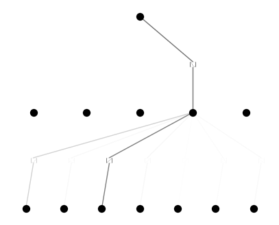
Step 15: Prune the Model
Remove unnecessary neurons and connections to simplify the model.
model.prune()
model.plot(mask=True)
model = model.prune()
model(dataset['train_input'])
model.plot()
Step 16: Continue Training with Symbolic Functions
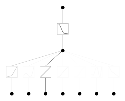
Set symbolic functions for activation functions and train the model to optimize it further.
model.train(dataset, opt="Adam", steps=50, lr=0.001)
model.plot()
mode = "auto"  ## Use automatic mode for setting symbolic functions
if mode == "manual":
    model.fix_symbolic(0,0,0,'sin')
    model.fix_symbolic(0,1,0,'x^2')
    model.fix_symbolic(1,0,0,'exp')
elif mode == "auto":
    lib = ['x','x^2','x^3','x^4','exp','log','sqrt','tanh','sin','abs']
    model.auto_symbolic(lib=lib)
#OUTPUT:
train loss: 3.52e-01 | test loss: 3.52e-01 | reg: 4.26e+00 : 100%|██| 50/50 [00:14<00:00,  3.57it/s]
fixing (0,0,0) with tanh, r2=1.0000007152557373
fixing (0,1,0) with tanh, r2=0.9095821380615234
fixing (0,2,0) with tanh, r2=1.0000007152557373
fixing (0,3,0) with tanh, r2=0.9738956093788147
fixing (0,4,0) with tanh, r2=0.7780349850654602
fixing (0,5,0) with sin, r2=0.5418534278869629
fixing (0,6,0) with sin, r2=0.4986622929573059
fixing (1,0,0) with tanh, r2=0.9674128890037537
Step 17: Train with Symbolic Functions
Train the model with symbolic functions to further optimize it.
model.train(dataset, opt="LBFGS", steps=50, lr=0.001)
symbolic_formula = model.symbolic_formula()[0][0]
print(symbolic_formula)
#OUTPUT:
train loss: 3.62e-01 | test loss: 3.62e-01 | reg: 4.81e+00 : 100%|██| 50/50 [00:06<00:00,  8.31it/s]
0.55 - 0.41*tanh(-0.43*sin(1.73*x_6 - 3.22) + 0.76*sin(5.94*x_7 + 0.13) + 7.05*tanh(0.85*x_1 + 0.44) + 10.55*tanh(5.33*x_2 - 9.2) + 6.09*tanh(4.72*x_3 + 5.35) + 2.84*tanh(0.1*x_4 - 0.54) + 2.5*tanh(1.38*x_5 - 6.28) + 14.07)
Step 18: Preprocess Test Data
Prepare the test data for making predictions.
test_df = test_data.drop(['PassengerId', 'Age', 'Cabin', 'Embarked'], axis=1)
test_df_scaled = scaler.transform(test_df)
test_input = torch.tensor(test_df_scaled, dtype=torch.float32)
Step 19: Ensure No NaNs in Test Data
Check that there are no NaN values in
the preprocessed test data.
assert not torch.isnan(test_input).any(), "NaNs found in test_input"
Step 20: Predict Survival Probabilities
Use the trained KAN model to predict survival probabilities for the test data.
y_pred_sub = model(test_input).detach().numpy()
Step 21: Convert Probabilities to Binary Outcomes
Apply a threshold to convert probabilities to binary outcomes.
threshold = 0.5
y_pred_sub = (y_pred_sub >= threshold).astype(int).flatten()  ## Ensure the predictions are a flat array
Step 22: Create Submission DataFrame
Organize the predictions into a DataFrame for submission to Kaggle.
sub = pd.DataFrame()
sub['PassengerId'] = test_data['PassengerId']
sub['Survived'] = y_pred_sub
Step 23: Display Submission DataFrame
Show the first few rows of the submission DataFrame.
print(sub.head())
   PassengerId  Survived
0          892         0
1          893         1
2          894         0
3          895         0
4          896         1
Conclusion
That's all folks, I was simply following the guide to training a model with pykan and hope you can perfect it by preprocessing the data better and optimizing hyperparameters, here are suggestions:
Feature Engineering:
- [Titles Extraction: Extract titles from names to add as a new feature.]
- [Family Size and IsAlone: Create new features to capture family relationships.]
Improved Missing Value Handling:
- [KNN Imputation: Use KNN imputer to fill missing values for
AgeandFare.]
Model Configuration:
- [Model Width and Grid: Enhance the model configuration for better learning capacity.]
Optimizer:
- [LBFGS: I Used LBFGS optimizer, try to see if you can get better results with a different optimizer]
Regularization:
- [Lambda and Entropy: Fine-tune regularization parameters to avoid overfitting.]
Written by
Anton Vice